Processing streaming data at scale presents a unique set of challenges that many organizations face daily. At Digital Turbine, we are handling massive volumes of real-time bidding data for DT Exchange, sometimes reaching 200 million events per minute. This calls for a robust infrastructure, often involving a significant number of machines. 

Here’s how our data pipeline looks like.

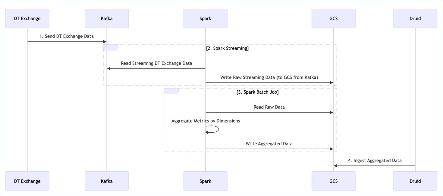
The pipeline leverages several key technologies, including Kafka for message queuing, Spark for both stream and batch processing, Google Cloud Storage (GCS) for intermediate and aggregated data storage, and Druid for fast data exploration. The process can be broken down into four main stages.

Stage 1. Data from DT Exchange is Sent to Kafka

The pipeline begins with the DT Exchange server, which acts as the primary source of raw data. As events or messages are generated, they are immediately published to a Kafka topic. Kafka serves as a distributed, high-throughput, and fault-tolerant message broker. This decouples the data producers (DT Exchange) from the consumers, ensuring that data can be reliably buffered and processed even if downstream systems experience temporary slowdowns or failures. Each message sent by the DT Exchange contains the initial dataset that will be processed through subsequent stages.

Stage 2. Real-Time Stream Processing with Spark Streaming

Downstream from Kafka, a Spark Streaming application continuously consumes messages from the designated Kafka topic. This component is responsible for the initial real-time processing of the incoming data. Upon reading a message, Spark Streaming performs any necessary preliminary transformations or enrichments and then writes the raw, unprocessed streaming data to a designated bucket in Google Cloud Storage (GCS). This ensures that all incoming data is captured and stored in its original form for auditing, reprocessing, or ad-hoc analysis.

Stage 3. Batch Data Aggregation with Spark

Periodically, a Spark batch job is initiated to process the raw data accumulated in GCS. This batch component performs more complex and computationally intensive operations:

• Reading Raw Data: The Spark job reads the raw streaming data that was previously landed in GCS by the Spark Streaming application.
• Aggregation: The core task of this stage is to aggregate metrics based on specified dimensions. This step transforms the granular raw data into a more summarized and structured format suitable for analytical querying.
• Writing Aggregated Data: Once the aggregation is complete, the Spark batch job writes the resulting aggregated dataset back to a different location within GCS. This aggregated data is optimized for efficient ingestion into analytical datastores.

Stage 4. Data Ingestion into Druid for Analytics

The final stage of the pipeline involves loading the aggregated data from GCS into Druid. Druid ingests the aggregated data, indexing it in a columnar format to enable low-latency querying. Once the data is available in Druid, it can be efficiently rendered in our GUI Dashboard, the DT Console. This allows end-users to explore trends, generate reports, and gain insights from the processed data.

Tackling the Triad of Data Engineering Challenges

Effective data engineering for large-scale systems often involves navigating a delicate balance between three core considerations: cost-effectiveness, operational stability, and data completeness. Successfully addressing these interconnected challenges is crucial for building reliable and sustainable data pipelines.

• Cost-Effectiveness at Scale: Efficiently managing resources is critical when dealing with large-scale streaming data. Optimizing resource allocation is essential to avoid excessive costs while maintaining the required processing power.
• Stability in a Dynamic Environment: Ensuring the stability of a streaming platform is essential. Various factors can threaten stability, including fluctuating data volumes, cloud infrastructure vulnerabilities, and the reliance on on-demand computing resources. In scenarios where revenue generation and critical decision-making depend on this data, maintaining stability is of utmost importance. Furthermore, since Kafka retention, due to high data volume, is limited to a few hours at most, the system must be capable of rapid recovery from infrastructure issues or data volume changes.
• Data Completeness for Reliability: Guaranteeing data completeness is vital for accurate reporting and analysis that directly impact stakeholders and business teams relying on this data for decision-making.

Optimizing Resource Allocation: Static Scaler

One strategy to tackle cost-effectiveness involves implementing a scaler with static configuration, meaning that scale action (up or down) will be based only on time of the day. This approach emphasizes the importance of understanding data behavior to optimize resource allocation. Recognizing patterns in data volume fluctuation, such as higher volumes on specific days of the week, is key. To this extent, operational periods are split into high-volume hours and low-volume hours.

We implemented this by using a Kubernetes Cron job that monitors the current time and allocates resources according to a predefined static configuration. This approach enables the system to scale resources up during peak operational times and scale them down during periods of lower activity, thereby optimizing costs. An example of the static scaler configuration is provided below.

from datetime import datetime
import requests

# Configuration
RUSH_START_HOUR = 18        # 6 PM
RUSH_END_HOUR = 2           # 2 AM

REGULAR_EXECUTORS = 5
REGULAR_CORES = 2
RUSH_EXECUTORS = 10
RUSH_CORES = 4

ARGOCD_API = "argocd.com"

def is_rush_hour():
    """Returns True if the current time is considered rush hour."""
    hour = datetime.utcnow().hour
    return hour >= RUSH_START_HOUR or hour < RUSH_END_HOUR

def get_scaled_resources():
    """Determines the right executor and core count based on time of day."""
    if is_rush_hour():
        return RUSH_EXECUTORS, RUSH_CORES
    else:
        return REGULAR_EXECUTORS, REGULAR_CORES

def scale_spark_application(app_name):
    """Sends a scale request to ArgoCD for the given Spark application."""
    executors, cores = get_scaled_resources()

    url = f"http://{ARGOCD_API}/api/v1/applications/{app_name}/scale"

    payload = {
        "spec": {
            "executor": {
                "instances": executors,
                "cores": cores
            }
        }
    }

    print(f"Scaling {app_name} → Executors: {executors}, Cores: {cores}")
    response = requests.post(url, json=payload, headers=headers)

    if response.ok:
        print("✅ Scale successful")
    else:
        print(f"❌ Scale failed: {response.status_code}")

# Run the scaler
scale_spark_application("my-spark-streaming-app")

‍Ensuring Stability: Dynamic Scaler

While implementing a Static Scaler was straightforward and yielded significant cost benefits, it primarily addresses predictable data patterns on "normal" days. However, streaming data volumes can be inherently unpredictable, influenced by events such as special promotions, seasonal variations, or unexpected infrastructure disruptions. In these instances, manual intervention was previously required to increase resources for the stream, a practice we aimed to eliminate.

To address these scenarios, we implemented another Kubernetes cron job called the "Dynamic Scaler." A Dynamic Scaler considers real-time factors like recent processing times, stream lag, and our consumer's maximum processing rate (the number of messages that can be read in one batch) to make intelligent decisions about scaling resources up or down. This dynamic adaptability enhances the resilience of streaming systems and promotes stability even under volatile conditions.

The following graph illustrates how the static and dynamic scalers manage resource allocation (number of Spark executors) over time.

At first, the Static Scaler is adjusting resources, scaling up during high-volume periods and down during low-volume periods. After a certain point, the Dynamic Scaler is activated, and the resources start fluctuating more frequently and dynamically in response to stream lag and other real-time metrics.

Ensuring Completeners: Tackling Late-Arriving Data

One of the issues that can impact completeness is late-arriving data, which means data arrives to stream after the next step in the pipeline has already started. In this case only partial data will be aggregated that will eventually lead to partial data in our reporting view, negatively affecting the decision-making of our business stakeholders working with reports. To address this, we iterated through a number of solutions.

Initial Approach: Fixed-Delay Scheduling 

Our initial assumption was that all data for a given hour would arrive within 15 minutes after that hour concluded. Based on this, we scheduled an Airflow DAG to trigger the aggregation process 15 minutes past each hour. However, this method proved problematic when streams experienced significant delays. Such delays forced manual intervention to disable the DAG and re-enable it only after the stream caught up, leading to time-consuming and error-prone operations.

Refinement: File Count Sensing 

Our second solution involved implementing an Airflow sensor. This sensor would monitor the hourly data folder in GCS and count the number of files. The pipeline would proceed only if no new files were written to the folder for a certain period, indicating that data for that hour was complete. While this approach covered most scenarios, it occasionally failed when the stream's processing time for a particular hour took longer than usual. In these instances, the sensor incorrectly detected data completion, allowing the pipeline to move to the next step with an incomplete dataset.

Enhanced Monitoring: Tracking Stream Progress with "Earliest Hour" Metric 

When the file count sensing solution proved insufficient, it became clear that better monitoring and more precise clarity regarding the stream's current state were necessary. Specifically, we needed a reliable way to understand which hour's data processing was truly complete.

To achieve this, we created a metric called "Earliest Hour." This metric provides an indication, at any given time, of the specific hour the stream is actively processing. For example, if the current time is 20:05, but the "earliest hour" metric shows that the stream is still working on data for hour 19, it signifies that the aggregation process for hour 19 cannot yet begin. Here's how it looks like.

On the graph, at 20:09, the stream began processing data for hour 20. This change in the "Earliest Hour" metric signals that all data for hour 19 has been completely processed, and the aggregation step for hour 19 can now safely proceed.

Definitive Solution: The "Seal File"

The insights gained from enhanced monitoring led us to our final and most robust solution. This approach uses an absolute indication of data completion, eliminating reliance on assumptions that could compromise the system's robustness.

We introduced the concept of a "Seal File". Leveraging the "Earliest Hour" metric, our Spark Streaming application can determine when all data for a specific hour has been processed and is no longer present in the active stream. At this point, the stream processing job writes an empty "Seal File" into the corresponding hourly folder in GCS. The existence of this file serves as an explicit signal to our downstream aggregation pipeline that all data for that particular hour has been successfully processed and is complete.

For example, if a "Seal File" exists in the GCS folder /day=2025-05-01/hour=06/, it signifies that the aggregation process for the data corresponding to 2025-05-01, 06:00, can begin.

This "Seal File" approach offers several key advantages:

• Timely Aggregation: Aggregation can be triggered as soon as the data for an hour is definitively complete.
• Resilience to Delays: System delays or fluctuations in stream processing time are automatically accommodated without halting or negatively impacting the aggregation process.
• Reduced Manual Intervention: The need for manual oversight and intervention is significantly minimized.
• Independent Validation: Data completeness for any given hour can be independently and reliably validated by checking for the presence of the Seal File.
• Cross-Team Synchronization: Other teams or downstream processes that depend on the completeness of this hourly data can also use the Seal File as a reliable signal to synchronize their own pipelines.

Conclusion: Addressing Streaming Data Challenges

In managing large-scale streaming data, a balanced approach is needed to address the primary challenges of cost, stability, and data completeness. Our efforts involved several key solutions:

• For cost-effectiveness, a Static Scaler was implemented to optimize resource use based on predictable, time-based data patterns.
• To improve stability, a Dynamic Scaler was introduced, allowing the system to adapt to unpredictable changes in data volume or other system events.
• To ensure data completeness and manage late-arriving data, the "Seal File" mechanism was established. This provides a clear signal for synchronizing downstream processes and helps ensure that aggregations use complete datasets.

Through the combination of these strategies, we developed a more efficient and dependable data pipeline for real-time data processing.

‍